Tutorials
Step-by-step guides for building workflows and applications with Texera.
This section provides complete, end-to-end tutorials that guide you through realistic Texera use cases — from building simple workflows to creating complex data analytics pipelines.
Texera tutorials help you learn by doing.
Each tutorial walks through a realistic workflow scenario, showing how to use Texera’s visual interface, operators, and execution engine to build and run data analytics applications.
🎯 What to Expect
The tutorials in this section will help you:
- Understand Texera’s workflow-based design step by step.
- Learn how to connect operators, configure parameters, and visualize results.
- Explore practical data use cases, such as text processing, joining datasets, and real-time analysis.
- Get comfortable with extending Texera by creating or modifying operators.
🧱 Structure
Each tutorial consists of:
- Goal Overview – what you’ll build and what problem it solves.
- Step-by-Step Instructions – detailed actions to complete the workflow.
- Key Takeaways – concepts and Texera features you’ll learn.
- Next Steps – related tutorials or examples to explore further.
🧭 Getting Started
If you’re new to Texera, start with the Getting Started guide to set up your local environment.
Once Texera is running, return here to begin working through the tutorials in order.
📚 Available Tutorials
This section will include multiple tutorials, such as:
- Building your first workflow
- Exploring data transformation operators
- Working with visualization tools
- Combining multiple datasets
- Extending Texera with custom operators
Each tutorial will include screenshots, sample data, and workflow files you can download and import into your Texera instance.
💡 Want to Contribute a Tutorial?
If you’ve built a useful workflow or want to help new users learn Texera, you can contribute your own tutorial:
- Create a Markdown page under
content/docs/tutorials/. - Include any relevant
.json workflow files or sample datasets. - Submit a pull request following our Contribution Guidelines.
Texera tutorials are designed to help you go from understanding concepts to building complete solutions — one workflow at a time.
1 - Guide for how to use Texera
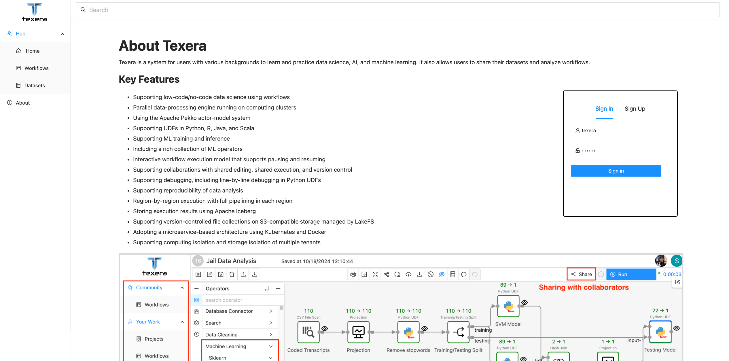
Texera is an open-source system that supports collaborative data science at scale using Web-based workflows. This page includes instructions on how to install the system as a developer and do a simple workflow.
Prerequisites
We assume you either went through Installing Apache Texera using Docker, or the Guide for Texera Developers. And Texera is up-and-running on your laptop.
Access Texera through Browser
Enter Texera’s URL on your browser to access Texera.
An admin account with username texera and password texera is pre-created by default. Input the username, password and click the Sign in button to login as the admin:
User Dashboard UI Overview
Once logged in, you should see the below page:
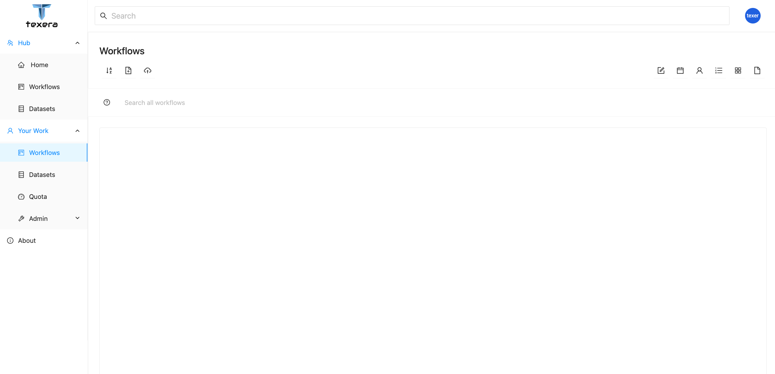
This is Texera’s dashboard page. On the left navigation bar, you can switch between different resource modules, including
Workflows for workflow managementDatasets for dataset managementQuota for checking the usage statisticsAdmin for managing users on the Texera system. This tab is only visible for system admins.
Workflow Workspace UI Overview
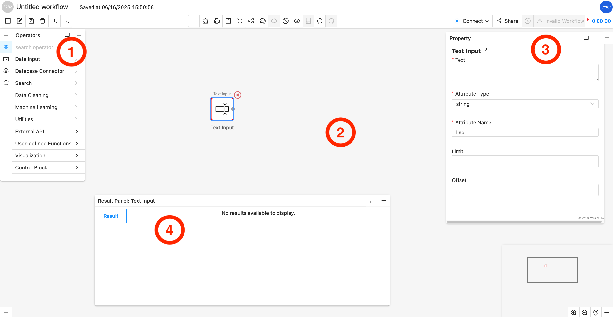
Operator Library/Menu:
It is separated into multiple dropdown menus based on the operator type, e.g., Source Operator, Search Operator, etc. You can drag and drop an operator from these dropdown menus onto the Workflow Canvas.
Workflow Canvas:
It is the main playground, where you can drag and drop Operators from the Operator Library onto it. Each operator is shown as a square box and connected with other operators with arrowed links which indicates the data flow.
Properties Editor Panel:
The panel will show up when you highlight a specific operator (by clicking on it) in the Workflow Canvas. You can customize the properties of the selected operator, for example, set the keyword for a filter. When the selected operator is configured correctly, a green ring will surround it; while a red ring usually indicates an error in configuration or connection to other operators.
Result Panel:
By default or when there is no result, it is hidden. You can click on the little UP arrow to expand this panel. When a workflow is finished running, the result panel will pop up with the data. You may slide up and down or left and right to view the data inside the panel.
2 - Create Dataset, upload data to it and use it in Workflow
This tutorial goes through the process of preparing data by creating dataset and creating a workflow to analyze data resided in the dataset using Texera.
More specifically, we are going to create a dataset named Sales Dataset which contains a file about the sales data of different types of merchandises for several countries. And the workflow will calculate the average sales per item type across different countries in Europe from the CountrySalesData.csv (Make sure the downloaded file is in .csv file extension). The sales data has been downloaded from eforexcel.com and has 100 rows of data.
We will first be creating a dataset and uploading the sales data to it. Then we will be creating a workflow on Texera Web UI to
- read the data from the file;
- filter the relevant data based on keywords;
- perform an aggregation.
1. Upload data by creating a Dataset
- Go to the Dataset tab and click the
dataset creation icon to start creating the datasaet - Name the dataset as
Sales Dataset, drag and drop the CountrySalesData.csv to the file uploading area - Click
Create, the dataset we just created, along with the preview of CountrySalesData.csv is shown.
2. Read data in Workflow
- On the left panel, go to the
environment tab and click Add Dataset to add the Sales Dataset to current workflow. CountrySalesData.csv will be available to be previewed and loaded to the workflow.
 '
' - Drag and drop a
CSV File Scan operator. On the right panel, input the file name CountrySalesData.csv and select the path from the drop down menu - Run the workflow, you should be able to see the loaded sales data.
3. Add operators to analyze data
3 - Guide to Use a Python UDF
What is Python UDF
User-defined Functions (UDFs) provide a means to incorporate custom logic into Texera. Texera offers comprehensive Python UDF APIs, enabling users to accomplish various tasks. This guide will delve into the usage of UDFs, breaking down the process step by step.
UDF UI and Editor
The UDF operator offers the following interface, requiring the user to provide the following inputs: Python code, worker count, and output schema.
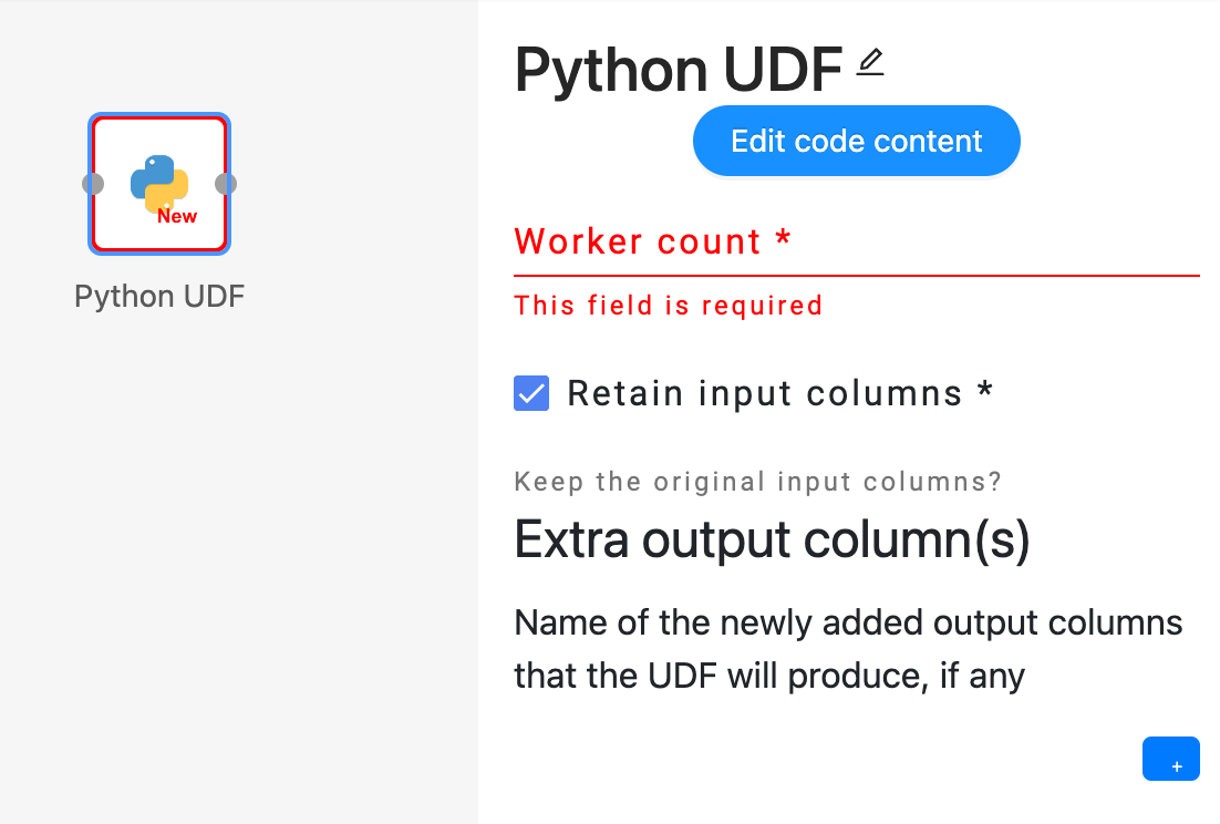
 Users can click on the “Edit code content” button to open the UDF code editor, where they can enter their custom Python code to define the desired operator.
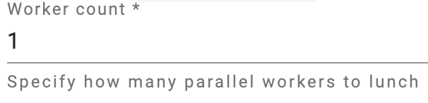 Users have the flexibility to adjust the parallelism of the UDF operator by modifying the number of workers. The engine will then create the corresponding number of workers to execute the same operator in parallel.
 Users need to provide the output schema of the UDF operator, which describes the output data’s fields.
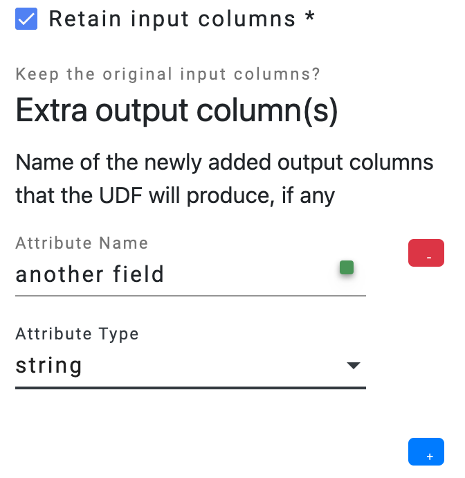
- The option
Retain input columns allows users to include the input schema as the foundation for the output schema. - The
Extra output column(s) list allows users to define additional fields that should be included in the output schema.
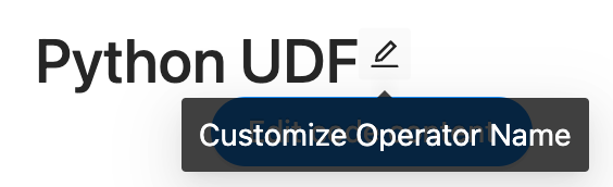 Optionally, users can click on the pencil icon located next to the operator name to make modifications to the name of the operator.
Operator Definition
Iterator-based operator
In Texera, all operators are implemented as iterators, including Python UDFs.
Concepturally, a defined operator is executed as:
operator = UDF() # initialize a UDF operator

... # some other initialization logic

# the main process loop
while input_stream.has_more():
    input_data = next_data()
    output_iterator = operator.process(input_data)
    for output_data in output_iterator:
        send(output_data)

... # some cleanup logic
Operator Life Cycle
The complete life cycle of a UDF operator consists of the following APIs:
open() -> None Open a context of the operator. Usually it can be used for loading/initiating some resources, such as a file, a model, or an API client. It will be invoked once per operator.process(data, port: int) -> Iterator[Optional[data]] Process an input data from the given port, returning an iterator of optional data as output. It will be invoked once for every unit of data.on_finish(port: int) -> Iterator[Optional[data]] Callback when one input port is exhausted, returning an iterator of optional data as output. It will be invoked once per port.close() -> None Close the context of the operator. It will be invoked once per operator.
Process Data APIs
There are three APIs to process the data in different units.
- Tuple API.
class ProcessTupleOperator(UDFOperatorV2):

    def process_tuple(self, tuple_: Tuple, port: int) -> Iterator[Optional[TupleLike]]:
        yield tuple_
Tuple API takes one input tuple from a port at a time. It returns an iterator of optional TupleLike instances. A TupleLike is any data structure that supports key-value pairs, such as pytexera.Tuple, dict, defaultdict, NamedTuple, etc.
Tuple API is useful for implementing functional operations which are applied to tuples one by one, such as map, reduce, and filter.
- Table API.
class ProcessTableOperator(UDFTableOperator):

    def process_table(self, table: Table, port: int) -> Iterator[Optional[TableLike]]:
        yield table
Table API consumes a Table at a time, which consists of all the tuples from a port. It returns an iterator of optional TableLike instances. A TableLike is a collection of TupleLike, and currently, we support pytexera.Table and pandas.DataFrame as a TableLike instance. More flexible types will be supported down the road.
Table API is useful for implementing blocking operations that will consume all the data from one port, such as join, sort, and machine learning training.
- Batch API.
class ProcessBatchOperator(UDFBatchOperator):

    BATCH_SIZE = 10

    def process_batch(self, batch: Batch, port: int) -> Iterator[Optional[BatchLike]]:
        yield batch
Batch API consumes a batch of tuples at a time. Similar to Table, a Batch is also a collection of Tuples; however, its size is defined by the BATCH_SIZE, and one port can have multiple batches. It returns an iterator of optional BatchLike instances. A BatchLike is a collection of TupleLike, and currently, we support pytexera.Batch and pandas.DataFrame as a BatchLike instance. More flexible types will be supported down the road.
The Batch API serves as a hybrid API combining the features of both the Tuple and Table APIs. It is particularly valuable for striking a balance between time and space considerations, offering a trade-off that optimizes efficiency.
All three APIs can return an empty iterator by yield None.
Schemas
A UDF has an input Schema and an output Schema. The input schema is determined by the upstream operator’s output schema and the engine will make sure the input data (tuple, table, or batch) matches the input schema. On the other hand, users are required to define the output schema of the UDF, and it is the user’s responsibility to make sure the data output from the UDF matches the defined output schema.
Ports
Input ports:
A UDF can take zero, one or multiple input ports, different ports can have different input schemas. Each port can take in multiple links, as long as they share the same schema.
Output ports:
Currently, a UDF can only have exactly one output port. This means it cannot be used as a terminal operator (i.e., operator without output ports), or have more than one output port.
1-out UDF
This UDF has zero input port and one output port. It is considered as a source operator (operator that produces data without an upstream). It has a special API:
class GenerateOperator(UDFSourceOperator):

    @overrides
    def produce(self) -> Iterator[Union[TupleLike, TableLike, None]]:
        yield
This produce() API returns an iterator of TupleLike, TableLike, or simply None.
See Generator Operator for an example of 1-out UDF.
2-in UDF
This UDF has two input ports, namely model port and tuples port. The tuples port depends on the model port, which means that during the execution, the model port will execute first, and the tuples port will start after the model port consumes all its input data.
This dependency is particularly useful to implement machine learning inference operators, where a machine learning model is sent into the 2-in UDF through the model port, and becomes an operator state, then the tuples are coming in through the tuples port to be processed by the model.
An example of 2-in UDF:
class SVMClassifier(UDFOperatorV2):


    @overrides
    def process_tuple(self, tuple_: Tuple, port: int) -> Iterator[Optional[TupleLike]]:

        if port == 0: # models port
           self.model = tuple_['model']

        else: # tuples port
           tuple_['pred'] = self.model.predict(tuple_['text'])
           yield tuple_
Currently, in 2-in UDF, “Retain input columns” will retain only the tuples port’s input schema.
4 - Guide to enable the LLM‐based Texera agent
This guide explains how to enable the AI agent feature in Texera. For detailed explanation about this feature, see https://github.com/apache/texera/pull/4020.
Prerequisites
- Already know how to setup Texera
- Python 3.10+
- API key from a supported LLM provider (e.g., Anthropic, OpenAI)
Step 1: Install LiteLLM
Run command:
pip install 'litellm[proxy]'
Set your LLM provider API key as an environment variable:
For Anthropic (Claude):
export ANTHROPIC_API_KEY=<your-anthropic-api-key>
For OpenAI:
export OPENAI_API_KEY=<your-openai-api-key>
You can set multiple API keys if you want to use models from different providers.
Step 3: Start LiteLLM Service
Start the LiteLLM proxy using the provided configuration:
litellm --config bin/litellm-config.yaml
By default, LiteLLM runs on http://0.0.0.0:4000.
To customize available models, edit bin/litellm-config.yaml. See LiteLLM documentation for more options. Also see LiteLLM Model Configuration for supported providers and model formats.
Step 4: Enable agent in Configuration
Modify common/config/src/main/resources/gui.conf to enable the agent feature:
 gui {
   workflow-workspace {
     # ... other settings ...

     # whether AI agent feature is enabled
-    copilot-enabled = false
+    copilot-enabled = true
   }
 }
The AccessControlService acts as a gateway between the frontend and LiteLLM. If LiteLLM is running on a different host or port, modify common/config/src/main/resources/llm.conf:
 llm {
   # Base URL for LiteLLM service
-  base-url = "http://0.0.0.0:4000"
+  base-url = "http://your-litellm-host:4000"

   # Master key for LiteLLM authentication
-  master-key = ""
+  master-key = "your-master-key"
 }
Alternatively, set environment variables:
export LITELLM_BASE_URL=http://your-litellm-host:4000
export LITELLM_MASTER_KEY=your-master-key
Step 6: Start Texera Services
Start the all Texera micro services, including the AccessControlService.
Done!
After opening any workflow, you should now see a robot icon at the bottom right. Click on it will expand a panel with all the available models:
5 - Guide to launch Lakekeeper as the RESTCatalog Service for Texera's workflow result storage
This guide goes through the process of setting up Lakekeeper, which can be used as the REST Catalog service for Texera’s workflow result storage.
For more information of why using RESTCatalog, see Issue #4126.
Prerequisites
- OS: macOS or Linux
- Already know how to setup Texera
- A running PostgreSQL instance
- An accessible S3 Bucket Endpoint
- awscli needs to be installed
Step 1: Install Lakekeeper
On macOS / Linux, run
Verify the installation by running:
Alternatively, you can download a pre-built binary from the https://github.com/lakekeeper/lakekeeper/releases and place it on your $PATH.
Step 2: Create a Database for Lakekeeper in Postgres
Create a database using the SQL script in Texera’s repository:
psql -f sql/texera_lakekeeper.sql
Edit the User Configuration section at the top of bin/bootstrap-lakekeeper.sh.
First, set the PostgreSQL connection URLs used by Lakekeeper:
-LAKEKEEPER__PG_DATABASE_URL_READ=""
-LAKEKEEPER__PG_DATABASE_URL_WRITE=""
+LAKEKEEPER__PG_DATABASE_URL_READ="postgres://<user>:<urlencoded_password>@<host>:5432/texera_lakekeeper"
+LAKEKEEPER__PG_DATABASE_URL_WRITE="postgres://<user>:<urlencoded_password>@<host>:5432/texera_lakekeeper"
If you have customized storage-related values in common/config/src/main/resources/storage.conf (for example, the bucket name, S3 endpoint, or MinIO credentials), check the below environment variables in the script and modify their values accordingly:
  # Storage settings — must stay in sync with storage.conf
  # if needed, update the default values after `:-` to match storage.conf
STORAGE_ICEBERG_CATALOG_REST_URI="${STORAGE_ICEBERG_CATALOG_REST_URI:-http://localhost:8181/catalog}"
STORAGE_ICEBERG_CATALOG_REST_WAREHOUSE_NAME="${STORAGE_ICEBERG_CATALOG_REST_WAREHOUSE_NAME:-texera}"
STORAGE_ICEBERG_CATALOG_REST_REGION="${STORAGE_ICEBERG_CATALOG_REST_REGION:-us-west-2}"
STORAGE_ICEBERG_CATALOG_REST_S3_BUCKET="${STORAGE_ICEBERG_CATALOG_REST_S3_BUCKET:-texera-iceberg}"
STORAGE_S3_ENDPOINT="${STORAGE_S3_ENDPOINT:-http://localhost:9000}"
STORAGE_S3_AUTH_USERNAME="${STORAGE_S3_AUTH_USERNAME:-texera_minio}"
STORAGE_S3_AUTH_PASSWORD="${STORAGE_S3_AUTH_PASSWORD:-password}"
Step 4: Run the Bootstrap Script
Run the following script in Texera repo:
bash bin/bootstrap-lakekeeper.sh
The script will:
- Start Lakekeeper if it’s not already running (on http://localhost:8181)
- Bootstrap the Lakekeeper server (creates the default project)
- Create the texera-iceberg bucket in MinIO if it doesn’t exist
- Register the texera warehouse with Lakekeeper, pointing at that bucket
Step 5: Verify
Check that Lakekeeper is healthy by running:
curl http://localhost:8181/health
You should see a JSON response with "health":"ok".
Verify that the warehouse has been created by running:
curl http://localhost:8181/management/v1/warehouse
You should see a warehouse in the response.
Step 6: Switch Texera to use the REST catalog
To make Texera actually use the Lakekeeper REST catalog you just set up, edit common/config/src/main/resources/storage.conf:
  storage {
      iceberg {
          catalog {
-             type = postgres
+             type = rest
              ...
          }
      }
  }
Done!
Lakekeeper is now your service of managing Iceberg RESTCatalog. Texera workflows that produce Iceberg results will write to the S3 bucket via the Iceberg RESTCatalog.
6 - Migrate a Jupyter Notebook to a Texera Workflow
This document provides guidelines on how to migrate a Jupyter notebook to a Texera workflow.
1. Overview
Jupyter Notebook is an open-source, browser-based environment for interactive computing that blends executable code with rich media in a single document. Work is organized into discrete cells that can be run individually, with each cell’s output persisted in the notebook.
A Texera workflow provides an operator-centric abstraction for data-science pipelines. A workflow is a directed acyclic graph (DAG) in which every node is an operator, such as CSV Scan, Projection, Filter, Aggregate, Python UDF, or ML Model, and an edge represents the flow of data between operators.
Migrating notebook code into Texera operators, then wiring those operators with links, transforms ad-hoc analyses into shareable, pipeline-oriented workflows that enable collaboration and scalable execution.
The notebook, dataset and workflow in this example are available on TexeraHub.
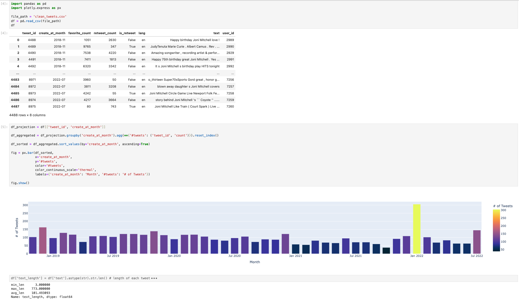
Notebook Overview
We will use a Tweet-Analysis notebook to demonstrate the migration process. The notebook has three cells:
import pandas as pd
import plotly.express as px

file_path = 'clean_tweets.csv'
df = pd.read_csv(file_path)
df
df_projection = df[['tweet_id', 'create_at_month']]
df_aggregated = df_projection.groupby('create_at_month').agg(**{'#tweets': ('tweet_id', 'count')}).reset_index()
df_sorted = df_aggregated.sort_values(by='create_at_month', ascending=True)
fig = px.bar(df_sorted,
             x='create_at_month',
             y='#tweets',
             color='#tweets',
             color_continuous_scale='thermal',
             labels={'create_at_month': 'Month', '#tweets': '# of Tweets'})
fig.show()
df['text_length'] = df['text'].astype(str).str.len()
length_stats = df['text_length'].agg(['min', 'max', 'mean'])
print(length_stats)
Below is the screenshot of the notebook after the execution:
2.1. Identify the data files and upload them to a Texera dataset
From cell 1, we see the notebook reads clean_tweets.csv.
#...
file_path = 'clean_tweets.csv'
df = pd.read_csv(file_path)
df
To let Texera read the same file, create a dataset in Texera, drag-and-drop the CSV file into it, and create a version:
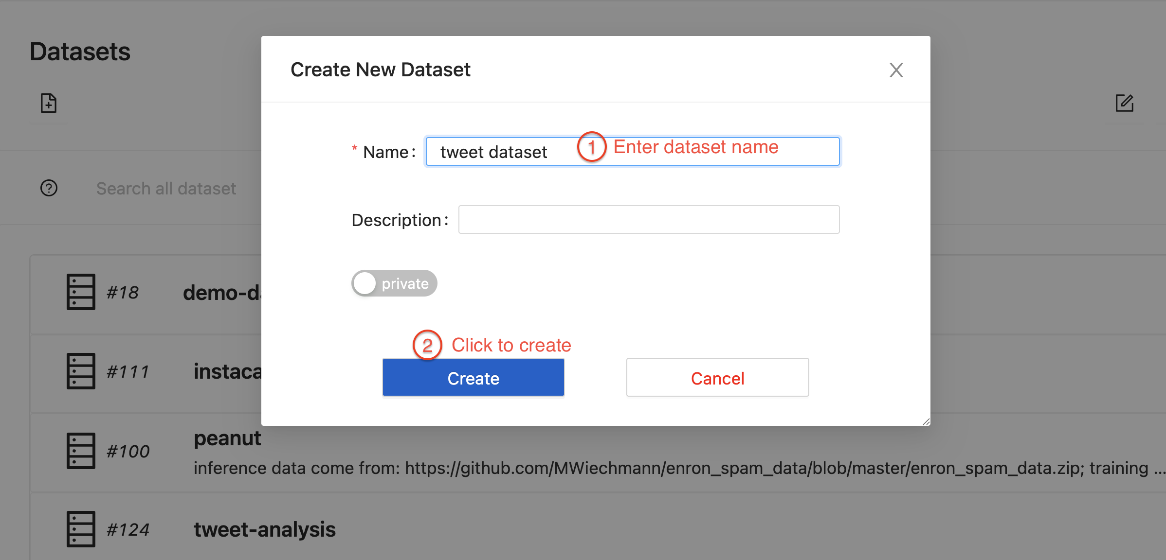
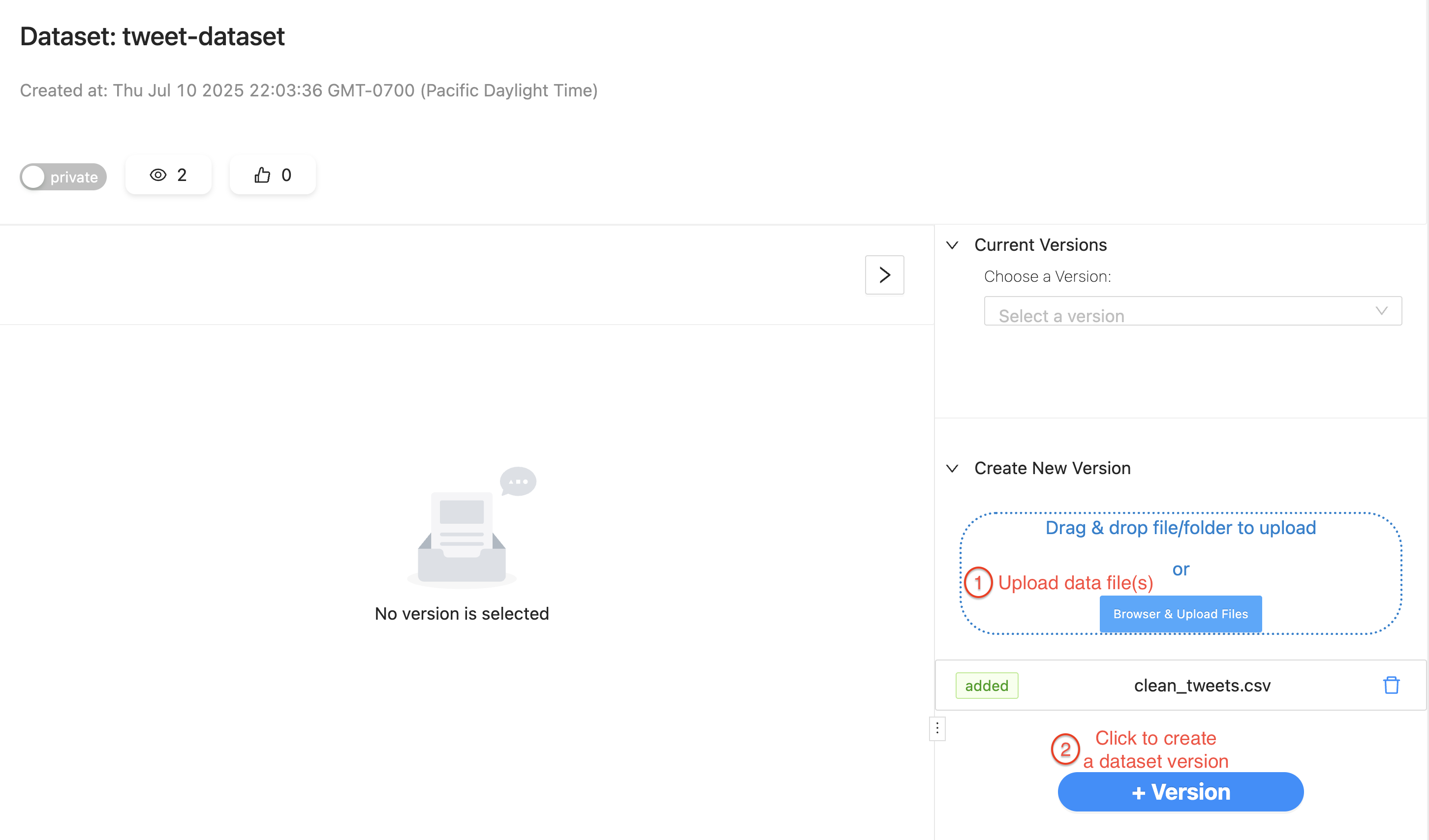
After the file is in a dataset, create a workflow and add a data-input operator that reads the file.
Because the file is CSV, we should use CSVFileScanOperator and specify the file path. Running the workflow should display the same table as Cell 1 in the result panel:
After this step, we have successfully converted cell 1 into a Texera operator.
2.3. Migrate data-processing logic into operators and links
Case 1: Use native operators for common processing logic
Cell 2 performs a sequence of operations after reading the data source: projection to keep only two columns, aggregation to calculate the number of tweets per month, sort based on count, and then visualizing using the bar chart:
df_projection = df[['tweet_id', 'create_at_month']]
df_aggregated = df_projection.groupby('create_at_month').agg(**{'#tweets': ('tweet_id', 'count')}).reset_index()
df_sorted = df_aggregated.sort_values(by='create_at_month', ascending=True)
fig = px.bar(df_sorted,
             x='create_at_month',
             y='#tweets',
             color='#tweets',
             color_continuous_scale='thermal',
             labels={'create_at_month': 'Month', '#tweets': '# of Tweets'})
fig.show()
These operations are very common in data science pipelines. And Texera provides several native operators that have the exact same functionalities and are easy to use:
- Projection operator →
df[['tweet_id', 'create_at_month']] - Aggregate operator →
groupby('create_at_month').agg(...).reset_index() - Sort operator →
sort_values(by='create_at_month', ascending=True) - Barchart operator →
px.bar(...)
Therefore, we can drag-n-drop these operators, connect them after the CSVFileScan. Running the workflow should display the same bar chart as in Cell 2.
Now we have successfully migrate cell 2 into Texera.
Case 2: Use UDF operators for complex processing logic
According to cell 3, a new column is added to the original tweet data table to represent the length of the text column. After that, min, max, mean of the text_length column are calculated.
df['text_length'] = df['text'].astype(str).str.len()
length_stats = df['text_length'].agg(['min', 'max', 'mean'])
print(length_stats.rename({'min': 'min_len', 'max': 'max_len', 'mean': 'avg_len'}))
For code that involves column addition/removal and other complex data operations, Texera supports UDF operators that allow users to write custom logic as an operator that processes the data.
In this example, we can add a PythonUDF operator after the CSVScanOperator. Inside the UDF we use TableAPI as it involves the table-level column addition. Since in the pytexera package, Table supports most of the pandas Dataframe APIs, we can simply adjust the code in Cell 3 and put it into UDF as the processing logic. There are two ways to show the final result:
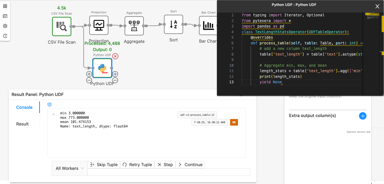
- Use
print statement in the UDF code block. The result will be shown in the “Console” tab:
from typing import Iterator, Optional
from pytexera import *
import pandas as pd
class TextLengthStatsOperator(UDFTableOperator):
    @overrides
    def process_table(self, table: Table, port: int) -> Iterator[Optional[TableLike]]:
        # add a new column text_length
        table['text_length'] = table['text'].astype(str).str.len()

        # Aggregate min, max, and mean
        length_stats = table['text_length'].agg(['min', 'max', 'mean'])
        print(length_stats)
        yield None
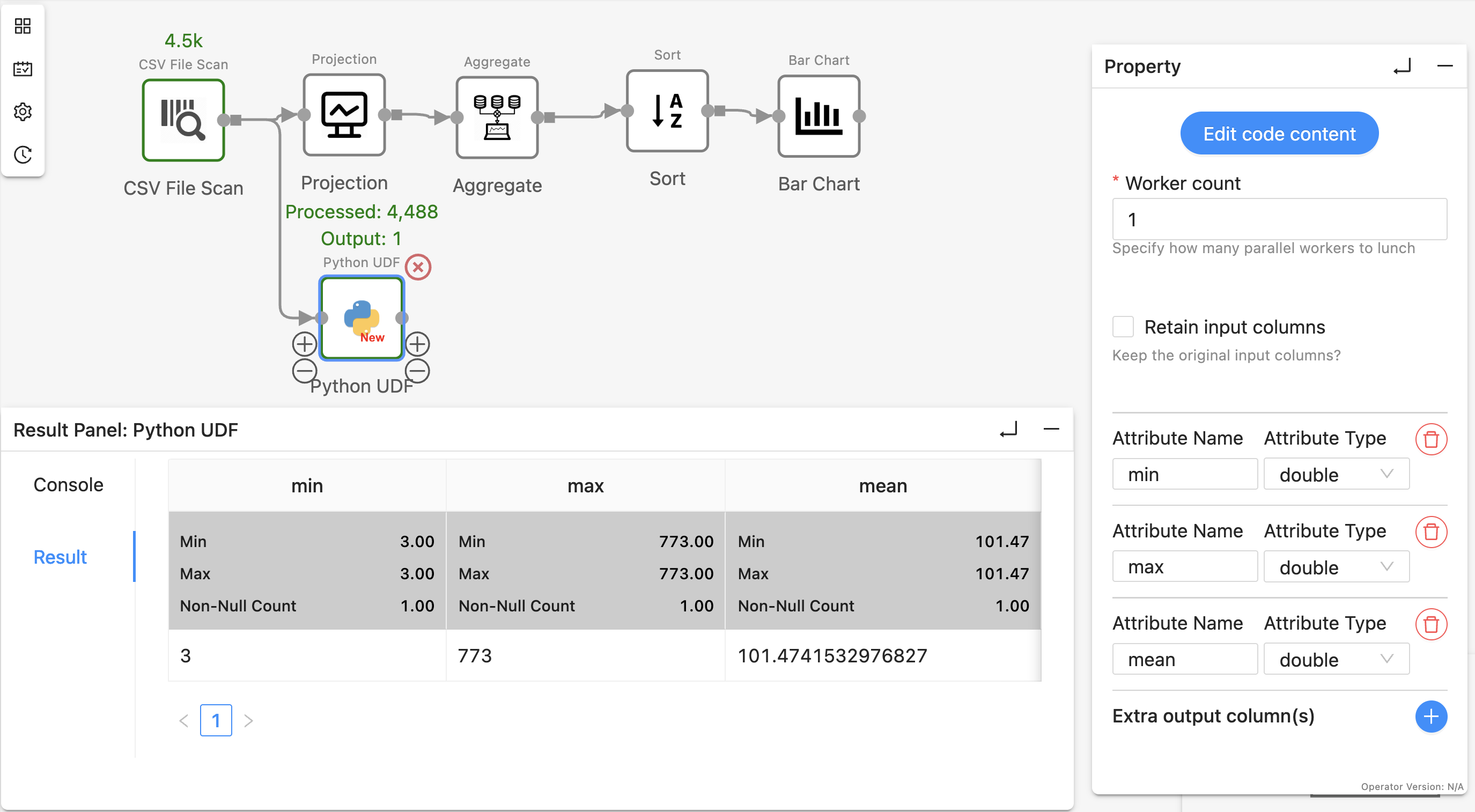
- Yield the result as a table with columns
min, max, and mean to the downstream. Make sure to declare the output schema in the operator panel. The result will be shown in the “Result” tab:
from typing import Iterator, Optional
from pytexera import *
import pandas as pd
class TextLengthStatsOperator(UDFTableOperator):
    @overrides
    def process_table(self, table: Table, port: int) -> Iterator[Optional[TableLike]]:
        # add a new column text_length
        table['text_length'] = table['text'].astype(str).str.len()

        # Aggregate min, max, and mean
        length_stats = table['text_length'].agg(['min', 'max', 'mean'])
        yield length_stats
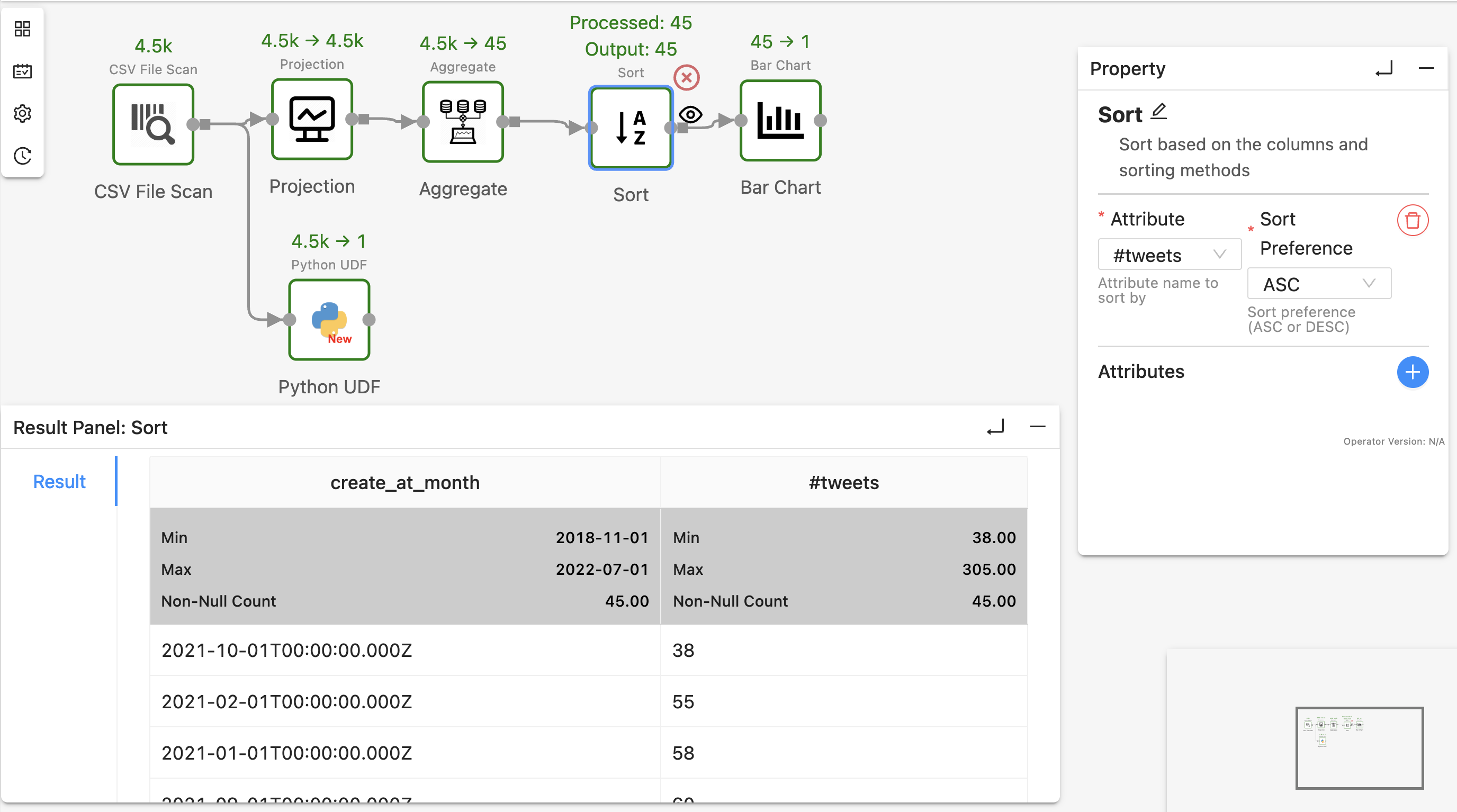
Step 4: Annotate some operators as ‘View Result’ to display the same results as Notebook
Jupyter displays the output of every cell, whereas Texera shows only sink-operator outputs by default.
To view intermediate results, for example, the results after SortOperator, right-click the operator, select “View Result” shown in the drop-down menu, and re-run the workflow:
Texera will now show the operator’s output in the result panel.
3. Tips
- Utilize Texera native operators as much as possible
Texera contains more than 110 built-in operators that cover data loading, cleaning, wrangling, visualization, and AI/ML. Replacing custom code with native operators makes workflows clearer and usually improves performance.
- Identify the data dependencies in the Python code in order to connect operators
In Texera, data flows along links. Before wiring operators, review the notebook to understand which variables feed which; then reproduce those dependencies via links so the executions matches the original notebook.